14. Seismic Facies Identification
This lab covers a challenging task: Seismic facies identification using machine learning. We’ll use data from the Seismic Facies Identification Challenge which is already preprocessed and can be used with little effort to apply our knowledge of efficient ML. Note that having carefully preprocessed data is a luxury we don’t typically have when working with experimental scientific data.
Our task is to classify volumetric stacked seismic data. Classification means that we have to decide what type of geological description applies to a given subsurface point. Stacked seismic data typically consists of an inline dimension, a crossline dimension, and a depth or time dimension. For more information, see the Introduction to 3-D seismic exploration section of the Society of Exploration Geophysicists wiki. In essence, seismic waves are reflected or manipulated at material interfaces. These effects are visible in the stacked seismic data which allows us to infer the corresponding subsurface material properties. In our dataset, a team of interpreters looked closely at the seismic data and labeled it for us. This allows us to learn from the labeled data and “interpret” seismic data on our own without years of training.
Keep in mind that we rely heavily on the interpreters to do a good job. Regardless of the quality of the data-driven ML method itself, we will not be able to outperform the interpreters in quality or correct errors. We would have to go a different way to do that. However, we can automate the interpreter’s work and probably do it much faster. For example, suppose an interpreter has labeled a small portion of a dataset for us. The ML-driven approach developed in this lab could allow us to automatically interpret the rest of the dataset.
14.1. Getting Started
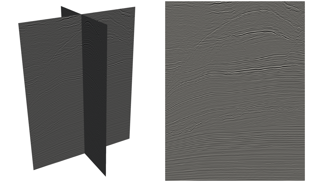
Fig. 14.1.1 Illustration of seismic data from the Seismic Facies Identification Challenge.
The dataset is available in the cloud directory seismic/data of the class.
It contains the labeled data, i.e. the files data_train.npz and labels_train.npz, which we use for training.
There are also two unlabeled files, data_test_1.npz and data_test_2.npz, which were used in the first and second round of the challenge respectively.
File |
nx |
ny |
nz |
dtype |
size (GiB) |
|---|---|---|---|---|---|
|
782 |
590 |
1006 |
||
|
|||||
|
|||||
|
Before we do any ML-related work, we’ll explore the dataset to get a good feel for it.
Tasks
Become familiar with the Seismic Facies Identification Challenge. Have a look at the Challenge Starter Kit
Fill in the missing entries in Table 14.1.1.
Visualize the data in
data_train.npzandlabels_train.npz. Slice the data to do this. Show slices in all dimensions, that is, slices normal to the x-, y- and z-direction. Create a plot that shows an xz-slice and a yz-slice at the same time
14.2. U-Net Architecture

Fig. 14.2.1 Illustration of the number of features involved and sizes in the U-Net type architecture of the code frame.
In 2015, the U-Net architecture was introduced in the context of biomedical image segmentation. Since then U-Nets have been applied to a wide range of scientific applications. U-Nets consist of an encoder that rapidly reduces the spatial size of the input, typically using max pooling steps to halve the image size in each step. At the same time, the convolutional blocks in the encoder increase the number of features.
The final output of the encoder is connected to the decoder through a convolutional bottleneck block. The decoder successively increases the spatial extent of the data by upsampling. Corresponding convolutional blocks in the decoder reduce the number of features. Furthermore, the encoder is connected to the decoder by skip connections.
In this task, we’ll use U-Net type networks for classification of seismic images. A working code base is provided in the cloud share of the class to get you over the initial hurdles. However, the code base is not optimized for either computational performance overall accuracy. Bottom line: This part is freestyle and you should follow your own ideas!
Tasks
Read the paper U-Net: Convolutional Networks for Biomedical Image Segmentation.
Briefly explain the following terms:
Max poopling
Upsampling by bilinear interpolation
Skip connection
Batch normalization
Train a U-Net network using data from the Seismic Facies Identification Challenge. Optimize your network! You are free to choose any approach you like. Document your ideas and results!