3. Bathymetry & Boundary Conditions

In this part of our project, we will first introduce bathymetry to our one-dimensional solver. Then, we will simulate a one-dimensional flow over a weir and study hydraulic jumps. Last, we run a one-dimensional tsunami simulation.

3.1. Non-zero Source Term

Bathymetry is the topography of the ocean and the most important part of the shallow water equation’s source term when simulating tsunamis. We use sea level as reference: Bathymetry in a dry cell (onshore) \(\mathcal{C}_i\) is zero or positive: \(b_i \ge 0\), a wet cell \(\mathcal{C}_j\) (offshore) has a negative value: \(b_j < 0\).

The introduction of bathymetry into the f-wave solver is comparably simple because it can be incorporated directly into the decomposition of the jump in the flux function:

(3.1.1)\[\Delta f - \Delta x \Psi_{i-1/2} = \sum_{p=1}^2 Z_p.\]

The term \(\Delta x \Psi_{i-1/2}\) summarizes[1] the effect of the bathymetry:

(3.1.2)\[\begin{split}\Delta x \Psi_{i-1/2} := \begin{bmatrix} 0 \\ -g (b_r - b_l) \frac{h_l+h_r}{2} \end{bmatrix}.\end{split}\]

Tasks

1. Extend the f-wave solver with support for bathymetry according to Eq. 3.1.1 and Eq. 3.1.2.

2. Implement an example which illustrates the effect of bathymetry in your extended solver. Note: You have to add bathymetry to the respective patches implementing the abstract class patches::WavePropagation as well. Also, ghost cells require a valid value for the bathymetry, i.e., set \(b_0 := b_1\) and \(b_{n+1} = b_n\).

[1]

Details can be found in: A wave propagation method for conservation laws and balance laws with spatially varying flux functions. D. S. Bale et. al., 2003.

3.2. Reflecting Boundary Conditions

The introduction of bathymetry naturally leads to the question of handling wetting and drying in near-shore areas, i.e., \(b(x) \approx 0\). The f-wave solver is not capable of handling wetting and drying. We will therefore impose two simplifications to keep our solver stable:

• Cells which are initially wet stay wet for the entire simulation: We assure each cell has enough water initially for the entire duration of a simulation. A fix for tsunami simulations will be introduced in Ch. 3.4.

• Cells which are initially dry stay dry for the entire simulation: At a wet-dry interface reflecting boundary conditions are used.

If a wave moves from a wet region towards the shore, we assume an infinitely high solid wall at the shore-line. This is equivalent to reflecting boundary conditions. Since no water is able to pass the shoreline, we have to ensure that the particle velocity at the boundary is zero.

Fig. 3.2.1 Wet-dry boundary for a wet cell \(\mathcal{C}_{i-1}\) and dry cell \(\mathcal{C}_i\).

Our finite volume scheme can have neighboring cells \(\mathcal{C}_{i-1}\) and \(\mathcal{C}_i\), where \(\mathcal{C}_{i-1}\) is wet and \(\mathcal{C}_{i}\) is dry. Fig. 3.2.1 illustrates this setting. As seen in the shock-shock example of Ch. 2.1, we obtain a middle state with zero particle velocity if we set an equal water height and an opposite-sign momentum in the dry cell. Additionally, setting the bathymetry in the dry cell to the value of the wet cell completes the setup of reflecting boundary conditions:

(3.2.1)\[\begin{split}h_{i} &:= h_{i-1} \\ (hu)_{i} &:= -(hu)_{i-1} \\ b_{i} &:= b_{i-1}\end{split}\]

Tasks

1. Implement reflecting boundary conditions as defined in Eq. 3.2.1.

2. Show that you obtain the Ch. 2.1’s one-sided solution of the shock-shock setup if you set \(q_l\) everywhere initially and use reflecting boundary conditions at the right boundary, and outflow boundary conditions at the left boundary. Note: Reflecting boundary conditions for the right boundary can be implemented through a ghost cell \(\mathcal{C}_{n+1}\) that is dry.

3.3. Hydraulic Jumps

This section illustrates the behavior of flows in a sub- and supercritical example. A lab-experiment is recorded in the video Hydraulics over a weir. In shallow water theory we can characterize this behavior by the Froude number:

\[F := \frac{u}{\sqrt{gh}}.\]

We call regions with \(F < 1\) subcritical, \(F \approx 1\) critical and \(F > 1\) supercritical. This definition matches the wave speeds of Ch. 1 in terms of the eigenvalues \(\lambda_{1/2} = u \mp \sqrt{gh}\). In the supercritical case the wave velocity relative to the fluid, i.e., \(\mp\sqrt{gh}\), is smaller than the velocity of the flow. Thus, information travels in one direction only and hydraulic jumps can occur. This behavior of flow is closely related to the subsonic, sonic and supersonic cases in acoustics.

The two following examples[2] set up a sub- and supercritical flow over a hump. We use the interval \((0, 25)\) as computational domain and outflow boundary conditions everywhere.

For the subcritical flow we use the following initial values:

(3.3.1)\[\begin{split}\begin{aligned} b(x) &= \begin{cases} -1.8 - 0.05 (x-10)^2 \quad &\text{if } x \in (8,12) \\ -2 \quad &\text{else} \end{cases}\\ h(x, 0) &= -b(x) \quad \text{if } x \in [0,25] \\ hu(x, 0) &= 4.42 \quad \text{if } x \in [0,25]. \end{aligned}\end{split}\]

For the supercritical flow we use the following initial values:

(3.3.2)\[\begin{split}\begin{aligned} b(x) &= \begin{cases} -0.13 - 0.05 (x-10)^2 \quad &\text{if } x \in (8,12) \\ -0.33 \quad &\text{else} \end{cases}\\ h(x, 0) &= -b(x) \quad \text{if } x \in [0,25] \\ hu(x, 0) &= 0.18 \quad \text{if } x \in [0,25]. \end{aligned}\end{split}\]

Tasks

1. Compute the location and value of the maximum Froude number for the subcritical setting given in Eq. 3.3.1 and the supercritical setting given in Eq. 3.3.2 at the initial time \(t=0\).

2. Implement both cases through the base class setup::Setup.h. \(t \in [0, 200]\) is a reasonable time window for your simulation.

3. Determine the position of the hydraulic jump (stationary discontinuity) in your supercritical solution and show that our f-wave solver fails to converge to the analytically expected constant momentum over the entire domain.

[2]

Details of the original benchmarks can be found in: Augmented Riemann solvers for the shallow water equations over variable topography with steady states and inundation. D. L. George, 2008.

3.4. 1D Tsunami Simulation

Now, with support for bathymetry in our Riemann solver, we can run our first one-dimensional simulations using field data. For this, we first extract input data for our solver from a Digital Elevation Model (DEM).

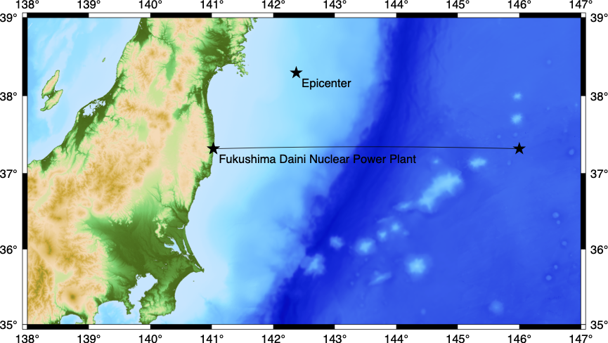
Fig. 3.4.1 Visualization of the GEBCO_2021 Grid and the one-dimensional domain as a line between the two points \(p_1=(141.024949, 37.316569)\) and \(p_2=(146.0, 37.316569)\). The epicenter of the March 11, 2011, M 9.1 Tohoku earthquake is north of the considered domain.

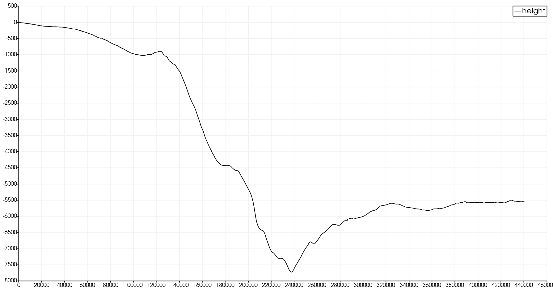
As illustrated in Fig. 3.4.1, we use the GEBCO_2021 Grid to extract the bathymetry profile between \(p_1=(141.024949, 37.316569)\) and \(p_2=(146.0, 37.316569)\). The Generic Mapping Tools’ function grdtrack is able to extract a 1D profile from a DEM. Fig. 3.4.2 shows the bathymetry data required by our solver for the one-dimensional domain.

Fig. 3.4.2 Visualization of the required bathymetry data, extracted from the GEBCO_2021 Grid.

Next, we extend our software by adding a simple CSV reader, which can parse the data for us. This reader is then used in a new setup setups::TsunamiEvent1d. The setup sets the following initial values for the water height \(h\), momentum \(hu\), and bathymetry \(b\):

(3.4.1)\[\begin{split}\begin{split} h &= \begin{cases} \max( -b_\text{in}, \delta), &\text{if } b_\text{in} < 0 \\ 0, &\text{else} \end{cases}\\ hu &= 0\\ b &= \begin{cases} \min(b_\text{in}, -\delta) + d, & \text{ if } b_\text{in} < 0\\ \max(b_\text{in}, \delta) + d, & \text{ else}. \end{cases} \end{split}\end{split}\]

\(b_\text{in}(x) \in \mathbb{R}\) is the bathymetry extracted from the DEM. \(d(x) \in \mathbb{R}\) is the vertical displacement, typically caused by a subduction-zone earthquake. In this task, we’ll use artificial displacement data, i.e., we assume:

\[\begin{split}d(x) = \begin{cases} 10\cdot\sin(\frac{x-175000}{37500} \pi + \pi), & \text{ if } 175000 < x < 250000 \\ 0, &\text{else}. \end{cases}\end{split}\]

The constant \(\delta \in \mathbb{R}^+\) avoids running into numerical issues due to missing support for wetting and drying in our solver. We will typically use \(\delta := 20\,\text{m}\) and apply reflecting boundary conditions whenever a wet cell neighbors a dry cell.

Tasks

1. Extract bathymetry data for the 1D domain, shown in Fig. 3.4.1, from the GEBCO_2021 Grid. Use a 250m sampling between the two points \(p_1\) and \(p_2\).

2. Extend the class tsunami_lab::io::Csv such that it can read your extracted bathymetry data.

3. Add a new setup setups::TsunamiEvent1d which uses your CSV reader and the artificial displacement to initialize your quantities as defined in Eq. 3.4.1.

4. Run and visualize the setup. What runup do you observe?

5. (optional) Modify the displacement! What are the impacts?