4. Two-Dimensional Solver

In this part of out project, we’ll cover the extension of our one-dimensional discretization to two spatial dimensions. Then, we’ll compare our two-dimensional solver to the one-dimensional one of the previous parts. After this chapter, we have all numerics at hand and will be able to conduct tsunami simulations in the following parts.

4.1. Dimensional Splitting

In their differential form, the two-dimensional shallow water equations are given as:

(4.1.1)$$\begin{array}{r}{\left[\begin{array}{c}h\\ hu\\ hv\end{array}\right]}_t+{\left[\begin{array}{c}hu\\ h{u}^2+\frac{1}{2}g{h}^2\\ huv\end{array}\right]}_x+{\left[\begin{array}{c}hv\\ huv\\ h{v}^2+\frac{1}{2}g{h}^2\end{array}\right]}_y=S(x,y,t).\end{array}$$

$t\in {\mathbb{R}}^{+}$ is time. $x\in \mathbb{R}$ and $y\in \mathbb{R}$ are the Cartesian coordinates. The quantities $q=[h,hu,hv{]}^T$ are given through the space-time dependent water height $h(x,y,t)$, the momentum in $x$-direction $hu(x,y,t)$ and the momentum in $y$-direction $hv(x,y,t)$. $F:=[hu,h{u}^2+\frac{1}{2}g{h}^2,huv{]}^T$ is the flux function in $x$-direction, and $G:=[hv,huv,h{v}^2+\frac{1}{2}g{h}^2{]}^T$ the one in $y$-direction. $g$ is the used gravity, usually we use $g:=9.80665\text{m}/{\text{s}}^2$. As for the one-dimensional shallow water equations, we only consider the space-dependent effect of bathymetry $B(x,y)$ in the source term $S(x,y)=[0,-gh{B}_x,-gh{B}_y{]}^T$.

The method of dimensional splitting allows us to apply our one-dimensional f-wave solver to the shallow water equations in two spatial dimensions. For this we split the two-dimensional problem into two one-dimensional ones which we solve after each other in so-called sweeps. The $x$-sweep is given as:

$$Q_{i,j}^{\ast }=Q_{i,j}^n-\frac{\mathrm{\Delta }t}{\mathrm{\Delta }x}(A^{+}\mathrm{\Delta }{Q}_{i-1/2,j}+A^{-}\mathrm{\Delta }{Q}_{i+1/2,j})\mathrm{\forall }i\in \{1,..,n\},j\in \{0,..,n+1\}.$$

The $y$-sweep is applied to the intermediate values $Q_{i,j}^{\ast }$ and defined as:

$$Q_{i,j}^{n+1}=Q_{i,j}^{\ast }-\frac{\mathrm{\Delta }t}{\mathrm{\Delta }y}(B^{+}\mathrm{\Delta }{Q}_{i,j-1/2}^{\ast }+B^{-}\mathrm{\Delta }{Q}_{i,j+1/2}^{\ast })\mathrm{\forall }i,j\in \{1,..,n\}.$$

As in the one-dimensional case, a cell ${\mathcal{C}}_i$ is influenced by all neighboring cells which are connected through the net-updates $A^{\pm }\mathrm{\Delta }{Q}_{i\mp 1/2,j}$ of the vertical edges $x_{i\mp 1/2,j}$ and $B^{\pm }\mathrm{\Delta }{Q}_{i,j\mp 1/2}^{\ast }$ of the horizontal edges $y_{i,j\mp 1/2}$. The time step restriction due to the CFL criterion for $\mathrm{\Delta }t$ is similar to the one-dimensional case but has to be true in the $x$- and $y$-sweep:

(4.1.2)$$\mathrm{\Delta }t<\frac{1}{2}\cdot \frac{\mathrm{\Delta }x}{{\lambda }_x^{\text{max}}}\wedge \mathrm{\Delta }t<\frac{1}{2}\cdot \frac{\mathrm{\Delta }y}{{\lambda }_y^{\text{max}}},$$

where ${\lambda }_x^{\text{max}}$ is the maximum eigenvalue appearing in the $x$-sweep and ${\lambda }_y^{\text{max}}$ the maximum eigenvalue in the $y$-sweep.

Note: We continue using our constant time step derived in the setup phase. This is valid as long as the CFL-criterion in Eq. 4.1.2 is satisfied for all time steps.

Tasks

1. Add support for two-dimensional problems to the solver. Implement dimensional splitting through a new class patches::WavePropagation2d. Change other parts of the software as required but keep supporting one-dimensional settings.

2. Implement a circular dam break setup in the computational domain $[-50,50{]}^2$ by using the following initial values:

   $$\begin{array}{r}\{\begin{array}{ll}[h,hu,hv{]}^T=[10,0,0{]}^T& \text{if }\sqrt{x^2+y^2}<10\\ [h,hu,hv{]}^T=[5,0,0{]}^T& \text{else}\end{array}\end{array}$$

3. Illustrate your support for bathymetry in two dimensions by adding an obstacle to the computational domain of the circular dam break setup.

4.2. Stations

When solving wave propagation problems, we are often times interested in output at specific points (or stations) of the computational domain. For a given station $s=(x,y)$, a quantity of interest, e.g., the deviation of the water colum from sea level ${\eta }_s(t)=h_s(t)+b_s(t)$ is then typically visualized, compared or analyzed. An example workload, often requiring per-station output, is given through verification and validation. In verification, we might run two solvers with the same inputs and compare the solution at a set of important stations. In validation, we would run our solver, and compare the resulting synthetic data to observed data.

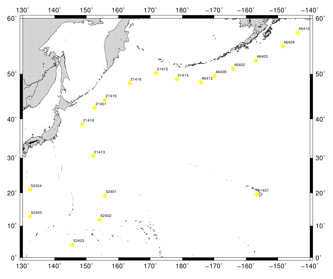
Fig. 4.2.1 Map of some DART stations in the Pacific. The stations are shown as yellow diamonds with their respective ids.

Fig. 4.2.1 shows a set of stations which are of interest for the 2011 M 9.1 Tohoku tsunami event. Specifically, the locations of some Deep-ocean Assessment and Reporting of Tsunamis (DART) stations are given. For these stations, we can access data of past tsunami events and thus do validation by comparing our numerical solutions to the measured data. An example of such a comparison is given in Fig. 4.2.2.

Fig. 4.2.2 Comparison of synthetic data (“Computed Solution”) to observed data (“Measured Data”) at DART station 21419 for the 2011 M 9.1 Tohoku tsunami event.

Tasks

1. Add a new class tsunami_lab::io::Stations which summarizes a collection of user-defined stations. Each station has a name and a location in space. All stations share the output frequency in seconds. The output for each station should be written in a separate ASCII-CSV file.

2. Find a suitable way to provide the names and locations of each stations to your solver. Further, implement a time step-independent output frequency for the stations. Keep in mind, that this runtime-configuration should be extensible and usable in later parts of the project. One possible solution are XML-based runtime configurations through the library pugixml.

3. Use a symmetric problem setup, e.g., a circular dam break problem, to compare your two-dimensional solver to your one-dimensional one at a set of stations.

4. (optional) Run a “convergence study”, i.e., use a synthetic setup and decrease the size of your grid cells. For example, for the computational domain $\mathrm{\Omega }=[0,100\text{m}{]}^2$ you could test mesh-spacings $h\in \{50,25,10,7.5,5,4,3,2,1\}$. Compare your solution at a set of points, what do you observe?