10. Single Cycle Processor

In theory we have all parts together and could start discussing the design of our own processors using SystemVerilog. Most importantly, we developed an NZCV-extended ALU in Section 7 which could build the centerpiece of our processor’s datapath. Our FPGA skills would then prove extremely helpful to conduct first tests and take our processor designs for a spin. If only there was some more time.. 😅

This chapter is split into two parts. First, in Section 10.1 we’ll study machine code and the underlying instruction encoding used in Arm architecture. An Arm processor is able to parse this machine code and behaves accordingly. Second, in Section 10.2 we’ll have a look at a very simple simulated Arm processor. This allows us to get an overview on how instructions are fetched, decoded and executed by a CPU.

10.1. Machine Code

In Section 9 we wrote simple functions in assembly language. Until this point the assembler took care of translating our assembly code to machine code. The machine code is how our executable programs are actually stored in memory. In this exercise we’ll manually translate a program from assembly language to machine code. This is nothing one would typically do in practice but crucial to understand the encoding of A64 instructions.

AArch64 has a fixed instruction size of 32 bits. Thus, a function with 10 instructions fits in 10 $\times$ 32 bits = 320 bits = 40 bytes. Logically an AArch64 processor reads bits 0-31, decodes the instruction and executes a corresponding operation. Next, the processor reads and decodes bits 32-63 and executes the respective operation. After that bits 64-95 are processed and so on. Branches operate differently from that. Here, potentially based on the result of a previous instruction, the processor might not simply jump to the next 32 bits but to another program position.

Optional Note

Certain recent extensions of the Arm architecture violate the idea that every operation is encoded in 32 bits. An example for more “complex” operations are those using prefix instructions of the Scalable Vector Extension (SVE). MOVPRFX (unpredicated), for example, allows us to perform a four-operand Fused-Multiply-Add (FMA4) operation. Effectively one would use two instructions, i.e., 2 $\times$ 32 bits = 64 bits, to realize FMA4. Some details on this are available from Fujitsu’s 2018 Hot Chips (HC30) presentation on A64FX.

Listing 10.1.1, Listing 10.1.2 and Listing 10.1.3 contain our usual structure: A C++ driver, a C reference implementation and the corresponding part in assembly language. This time, however, the assembly code is already provided in Listing 10.1.3’s function machine_code_asm_0. Our goal is perform the manual translation of every single human-readable instruction to machine code. This allows us to re-implement the function in machine_code_asm_1 by using only machine code.

We’ll do this by looking up the instructions of machine_code_asm_0 in the ISA and writing down the respective machine code in Table 10.1.2. Good news, you are in luck! Table 10.1.1 already contains most of the relevant links to the ISA and a short form of respective instruction encoding. Only SUBS (immediate) is missing.

Listing 10.1.1 C++ driver for the machine code example.

#include <cstdint>
#include <cstdlib>
#include <iostream>

extern "C" {
  uint64_t machine_code_c();
  uint64_t machine_code_asm_0();
  uint64_t machine_code_asm_1();
}

int main() {
  uint64_t l_result_c = 0;
  uint64_t l_result_asm_0 = 0;
  uint64_t l_result_asm_1 = 0;

  // machine_code_c
  std::cout << "### calling machine_code_c ###" << std::endl;
  l_result_c = machine_code_c();
  std::cout << l_result_c << std::endl;

  // machine_code_asm_0
  std::cout << "### calling machine_code_asm_0 ###" << std::endl;
  l_result_asm_0 = machine_code_asm_0();
  std::cout << l_result_asm_0 << std::endl;

  // machine_code_asm_1
  std::cout << "### calling machine_code_asm_1 ###" << std::endl;
  l_result_asm_1 = machine_code_asm_1();
  std::cout << l_result_asm_1 << std::endl;

  return EXIT_SUCCESS;
}

Listing 10.1.2 C kernel which provides the high-level reference of our machine code example.

#include <stdint.h>

uint64_t machine_code_c() {
  uint64_t l_tmp_0 = 0;
  uint64_t l_tmp_1 = 0;
  uint64_t l_tmp_2 = 0;

  l_tmp_0 = l_tmp_0 + 5;

  while( 1 ) {
    l_tmp_1 = l_tmp_1 + 3;
    l_tmp_2 = l_tmp_2 + 7;

    l_tmp_0--;
    if( l_tmp_0 == 0 ) break;
  }

  l_tmp_0 = l_tmp_1 + l_tmp_2;

  return l_tmp_0;
}

Listing 10.1.3 Assembly kernel machine_code_asm_0 which serves as the reference implementation.

        .text
        .align 4
        .type   machine_code_asm_0, %function
        .global machine_code_asm_0
machine_code_asm_0:
        eor x0, x0, x0
        eor x1, x1, x1
        eor x2, x2, x2

        adds x0, x0, #5

my_loop:
        adds x1, x1, #3
        adds x2, x2, #7

        subs x0, x0, #1
        b.ne my_loop

        adds x0, x1, x2

        ret
        .size   machine_code_asm_0, (. - machine_code_asm_0)

        .text
        .align 4
        .type   machine_code_asm_1, %function
        .global machine_code_asm_1
machine_code_asm_1:
        // TODO: implement machine-code version
        .size   machine_code_asm_1, (. - machine_code_asm_1)

Table 10.1.1 Instruction encodings for the function `machine_code_asm_0`.
Instruction	Instruction Encoding
EOR (shifted register)	`f100 1010 ss0m mmmm iiii iinn nnnd dddd`
ADDS (immediate)	`f011 0001 0hii iiii iiii iinn nnnd dddd`
SUBS (immediate)	`???? ???? ???? ???? ???? ???? ???? ????`
B.cond	`0101 0100 iiii iiii iiii iiii iii0 cccc`
ADDS (shifted register)	`f010 1011 ss0m mmmm iiii iinn nnnd dddd`
RET	`1101 0110 0101 1111 0000 00nn nnn0 0000`

Table 10.1.2 Instructions written in assembly language and machine code for the function `machine_code_asm_0`.
Assembly Language	Machine Code (binary)	Machine Code (hex)
`eor x0, x0, x0`	`1100 1010 0000 0000 0000 0000 0000 0000`	`ca000000`
`eor x1, x1, x1`	`1100 1010 0000 0001 0000 0000 0010 0001`	`ca010021`
`eor x2, x2, x2`
`adds x0, x0, #5`
`adds x1, x1, #3`
`adds x2, x2, #7`
`subs x0, x0, #1`
`b.ne my_loop`
`adds x0, x1, x2`
`ret`	`1101 0110 0101 1111 0000 0011 1100 0000`	`d65f03c0`

Tasks

Complete Table 10.1.1 by looking up the instruction encoding of SUBS (immediate). Use a short format similar to the already provided one for ADDS (immediate).
Complete Table 10.1.2 by providing the binary and hexadecimal machine code of all instructions.
Hint
- The immediate imm19 of B.cond is in two’s complement representation. This means that 111 1111 1111 1111 1111 represents the decimal value -1.
- A description of the condition codes is available from the Arm Architecture Reference Manual Armv8, for A-profile architecture in Chapter C1.2.4 / Table C1-1.
Implement the function machine_code_asm_1 in Listing 10.1.3 by only using your hex version of the machine code.

Hint

The directive .inst allows you to provide a numeric opcode in your assembly code. For example, for the first instruction eor x0, x0, x0 one may alternatively write .inst 0xca000000.

Hint

You may assemble a single instruction by using the tool llvm-mc. For example, you could use the following command to assemble the instruction adds x0, x0, #5:

echo "adds x0, x0, #5" | llvm-mc -triple=aarch64 --show-encoding

Conversely, you may also use llvm-mc to disassemble a single instruction. For example, to disassemble 0xb1001400 you could use:

echo "0x00 0x14 0x00 0xb1" | llvm-mc -triple=aarch64 -disassemble --show-encoding

10.2. ISA Simulator

This subsection studies how our programs are interpreted and executed by a (very) simple processor. For this we’ll use the Graphical Micro-Architecture Simulator. The simulator supports a subset of the Armv8-A ISA called the LEGv8 instructions. All instructions used in Section 10.2 are part of LEGv8.

The real value of the simulator lies in the visualization of the implemented processors’ register states, control and data paths. In this subsection we’ll use the single-cycle execution mode of the simulator. This means that within one cycle the processor fetches an instruction from instruction memory, decodes it and executes it entirely.

Optional Note

Modern processors work on many instructions in parallel and often require more than a single cycle to execute a single instruction. One heavily used mechanism for Instruction-Level Parallelism (ILP) is called pipelining. You may switch to a pipelined variant of the simulator by selecting it as “Execution Mode”.

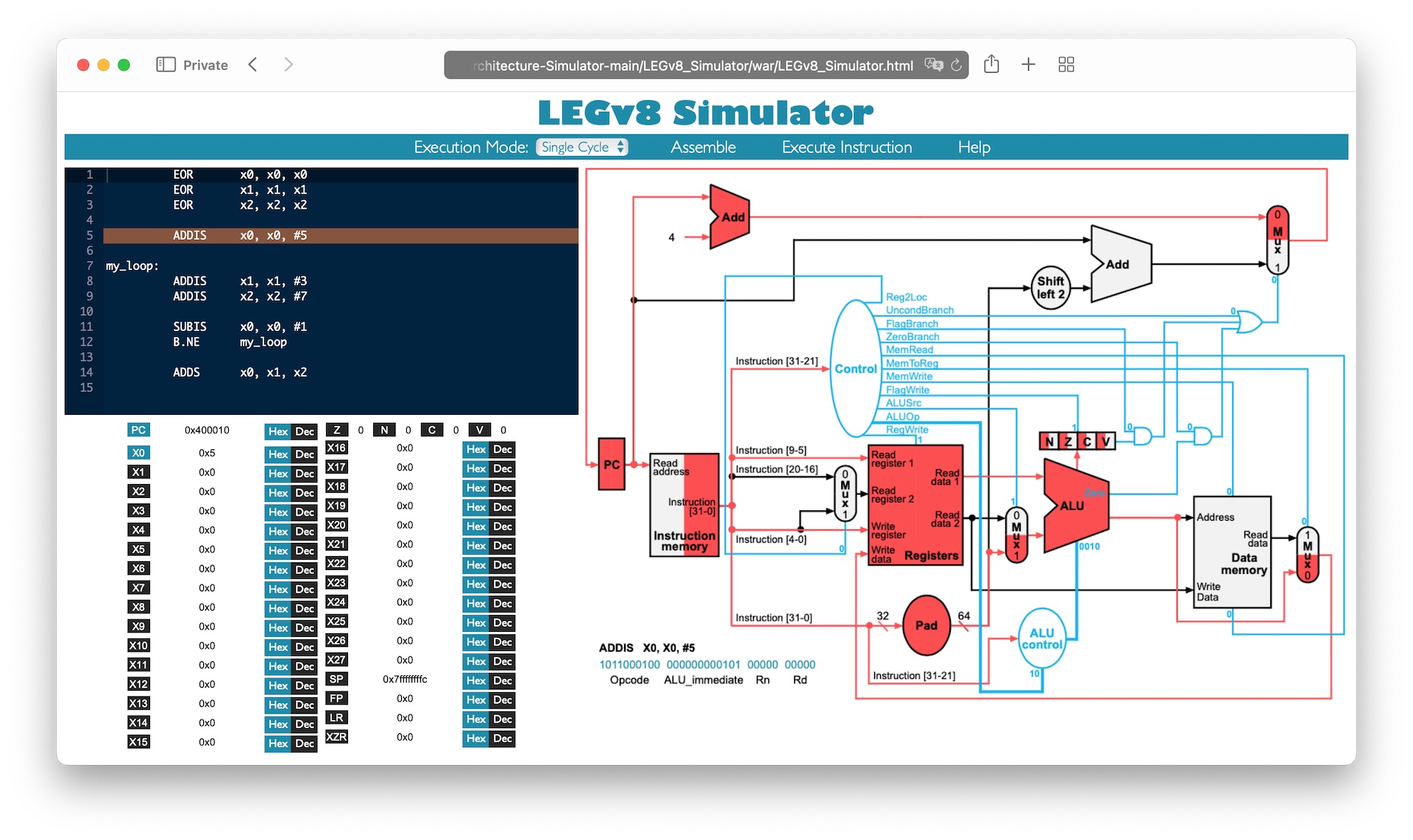
../_images/legv8_simulator_small.jpg — Fig. 10.2.1 Arm’s Graphical Micro-Architecture Simulator (v1.0.0) in action. Shown is the simulated data path and control for the fourth instruction `adds x0, x0, #5` of the code (excluding `ret`) in Listing 10.1.3. Active parts of the datapath are highlighted in red. Only the left side of the NZCV condition flags is highlighted in red to indicate that these are written.

Fig. 10.2.1 shows the active parts of the datapath when executing the instruction adds x0, x0, #5 in red. Further, respective bits of the control are given. We see that the current value of the Program Counter (PC) is used as an input to a red adder which uses the value 4 as second input. The output of the adder is then passed on to a multiplexer which selects the output of this adder since the multiplexer’s control bit is 0. The multiplexer’s output is the program counter’s value in the next cycle. In summary, the program counter is simply incremented by 4 when executing adds x0, x0, #5 as we would expect based on the discussion in Section 10.1.

For the remainder of this subsection we’ll study how the branches in the execution of the code in Listing 10.1.3 manipulate the program counter.

Tasks

Use the Graphical Micro-Architecture Simulator to assemble the code in Listing 10.1.3. Exclude the ret instruction. Use addis instead of adds and subis instead of subs when entering the assembly code. Run the code until you reach instruction addis x0, x1, x2. Provide screenshots with ascending names, i.e., bne_0.png, bne_1.png and so on, which show the visualized processor after every executed conditional branch.
Briefly describe the changes of the program counter after every execution of a branch instruction. Briefly explain the reasons for the observed changes.